BLR Models#
brains already encapsulates several BLR dynamical models detailed below. To specify those models in
running, edit the option “FlagBLRModel” in the parameter file (see Parameter File).
Broad-line regions are generally assumed to be composed of a larg number of point-like clouds. These clouds respond to the central ionizing continuum and emit broad emission lines.
BLR coordinate and observer’s coordinate#
The BLR coordinate is adopted to be left-handed (see Fig.1). The x-axis is set to be along the line of sight and the positive x-axis points to the observer. That is to say, a positive velocity in the BLR’s coordinate corresponds to a blus-shift velocity in observer’s coordinate.
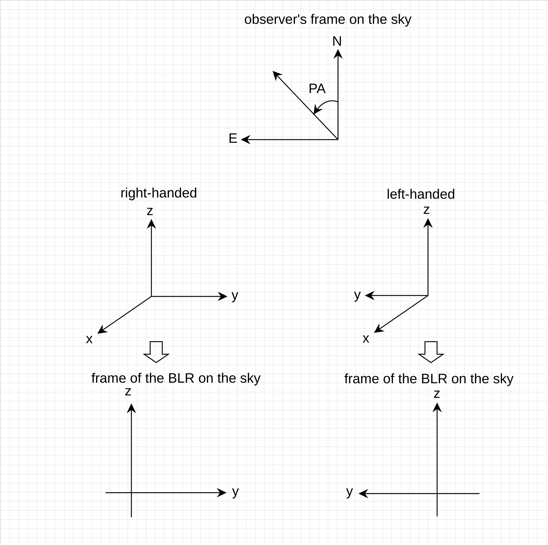
Fig.1 The coordinate frames. X-axis is the along the line of sight and positive x-axis points to the observer. Left-handed coordinate of the BLR is preferred, which is consistent with the coordinate frame of the observer. However, for axisymmetric BLRs, the two types of coordinate frames are indistinguishable.#
BLR model 1#
This model is from Brewer et al. (2011). Clouds’ distribution has a disk-like shape (see the figure) and is axis-symetric.
Radial distribution: \(\Gamma\)-distribution
\[\Gamma(r|\alpha, \theta) = \frac{1}{\Gamma(\alpha)\theta^{\alpha-1}}r^{\alpha-1}\exp\left(-\frac{r}{\theta}\right)\]Dynamics: clouds’ orbital angular momentum and energy are randomly assigned following distributions
\[\begin{split}E = \left(\frac{1}{1+\exp(-\chi)}\right)E_{\rm min},~~~ E_{\rm min}=-\frac{GM_\bullet}{r}, ~~~\chi\sim N(0, \lambda^2)\\ p(L)\sim \exp\left(-\frac{|L|}{\lambda L_{\rm max}}\right),~~~ |L| < L_{\rm max} = \sqrt{2r^2\left(E+\frac{GM_\bullet}{r}\right)}\end{split}\]Emissivity: anisotropic prescription
\[w(\phi) = \frac{1}{2} + \kappa \cos\phi\]where \(\phi\) is the angle between the observer’s line of sight to the central ionizing source and the cloud’s line of sight to the central source.

Fig.2 Schematic of a disk-like broad-line region (Li et al. 2013).#
BLR model 2#
The radial distribution and emissivity are the same as model 1. The dyanmics of clouds are modeled in the orbital plane as
where \(V_{\rm circ}=\sqrt{GM_\bullet/r}\) is the circular velocity.
BLR model 3#
Radial distribution: power-law distribution
\[\rho(r|\alpha) = \rho_0 \left(\frac{r}{r_0}\right)^{-\alpha},~~~~r_{\rm in} < r < r_{\rm out}\]Dynamics: Keplerian motion and inflow/outflow.
\[\boldsymbol{v} = V_{\rm Kep}\boldsymbol{e_{\theta}} + \xi \sqrt{\frac{2GM_\bullet}{r}} \boldsymbol{e_{r}}\]
BLR model 4#
This model is the same as model 3, except for the dynamics
BLR model 5#
Radial distribution: double power-law distribution.
The dyanmics and emissivity are the same as model 6.
BLR model 6#
This is compatible with Pancoast et al. (2014)’s model.
Radial distribution: \(\Gamma\)-distribution
\[\Gamma(r|\alpha, \theta) = \frac{1}{\Gamma(\alpha)\theta^{\alpha-1}}r^{\alpha-1}\exp\left(-\frac{r}{\theta}\right)\]Dynamics: A fraction \(f_{\rm ellip}\) of clouds have bound elliptical Keplerian orbits and the remaining fraction \((1-f_{\rm ellip})\) is either inflowing \((0 < f_{\rm flow} < 0.5)\) or outflowing \((0.5 < f_{\rm flow} < 1)\).
For elliptical orbits, the radial and tangential velocities are drawn from Gaussian distributions centered around a point \((v_r, v_\phi) = (0, v_{\rm circ})\) with standard deviations \(\sigma_{\rho,\rm circ}\) and \(\sigma_{\Theta,\rm circ}\), respectively. Here, \(v_{\rm circ}=\sqrt{GM_\bullet/r}\) is the local Keplerian velocity.
For inflowing/outflowing clouds, velocities are drawn similarly from Gaussian distributions centered around points \((v_r, v_\phi) = (\pm \sqrt{2} v_{\rm circ}, 0)`\) with standard deviations \(\sigma_{\rho,\rm rad}\) and \(\sigma_{\Theta,\rm rad}\), where “+” corresponds to outflows and “−” corresponds to inflows.
Emissivity: anisotropic prescription
\[w(\phi) = \frac{1}{2} + \kappa \cos\phi\]where \(\phi\) is the angle between the observer’s line of sight to the central ionizing source and the cloud’s line of sight to the central source.
BLR model 7#
This is the shadowed model in Li et al. (2018).

Fig.3 Schematic of a disk-like broad-line region with two zones (Li et al. 2018).#
BLR model 8#
A disk wind model from Shlosman & Vitello (1993).

Fig.4 Schematic of a disk wind model (figure credit: Higginbottom et al. 2013).#
In the cylindrical coordinate, the wind stream line have an angle as
where \(r_0\) is the root point of the stream line. The velocity along the stream line is
where \(l\) is the distance along the stream line, \(R_v\) is the scale length, \(v_0\) is the initial velocity, and \(v_\infty\) is the terminal velocity defined to be
The velocity components are
The azimuthal velocity is given by assuming conservations of the angular momentum
The density along the stream line is given by
where \(\dot m\) is the mass-loss rate at the root of the stream line.
BLR model 9#
This is the model adopted in the spectroastrometric modeling on 3C 273 by GRAVITY Collaboration (2018).
Radial distribution: \(\Gamma\)-distribution
\[\Gamma(r|\alpha, \theta) = \frac{1}{\Gamma(\alpha)\theta^{\alpha-1}}r^{\alpha-1}\exp\left(-\frac{r}{\theta}\right)\]Dynamics: circular Keplerian motion,
\[V_{\rm Kep} = \sqrt{\frac{GM}{r}}.\]Emissivity: isotropic prescription.
References#
Brewer, B. et al. 2011, ApJL, 733, 33
GRAVITY Collaboration et al. 2018, Nature, 563, 657
Higginbottom, N. et al. 2013, MNRAS, 436, 1390
Li, Y.-R. et al. 2013, ApJ, 779, 110
Li, Y.-R. et al. 2018, ApJ, 869, 137
Pancoast, A. et al. 2014, MNRAS, 445, 3055
Shlosman I., Vitello P., 1993, ApJ, 409, 372