Nested Sampling

brains employs the diffusive nested sampling algorithm developed by Brendon J. Brewer (eggplantbren/DNest3). We write a C version of the algorithm, dubbed as CDNest. CDNest needs to input some options.

The format of option file for CDNest looks like as follows:

# File containing parameters for DNest
# Put comments at the top, or at the end of the line.
# Lines beginning with '#' are regarded as comments.

NumberParticles          2
NewLevelIntervalFactor   2
ThreadStepsFactor        2
MaxNumberSaves           10
PTol                     0.1

# Full options are:
# NumberParticles          2
# NewLevelIntervalFactor   2
# SaveIntervalFactor       2
# ThreadStepsFactor        10
# MaxNumberLevels          0
# BacktrackingLength       10.0
# StrengthEqualPush        100.0
# MaxNumberSaves           10000
# PTol                     0.1

The option file for continuum reconstruction is OPTIONSCON, for 1d RM is OPTIONS1D, and for 2d RM is OPTIONS2D. brains will automatically reads these options appropriately.

Lines beginning with ‘#’ are regarded as comments. The meaning of these options are:

• NumberParticles constrols the number of particles for each core.

• MaxNumberSaves constrols the number of saves, namely, the number of output parameter samples.

• PTol constrols likelihood tolerance in loge.

• ThreadStepsFactor constrols the steps that each core run before all cores communicate, i.e., ThreadStep=ThreadStepsFactor * NumberParticles * NumberParameters.

• NewLevelIntervalFactor constrol the steps for creating a new likelihood level, i.e., NewLevelInterval=NewLevelIntervalFactor * NumberCores * ThreadSteps.

• SaveIntervalFactor controls the steps that all cores run for saving a sample, i.e., SaveInterval = SaveIntervalFactor * NumberCores * ThreadSteps.

• BacktrackingLength controls the backforward tracking length (lambda in Brewer’s paper).

• StrengthEqualPush controls strength to force equal push (beta in Brewer’s paper).

There is not a general rule to set the values of options. Sufficiently large values will work better, but also will cause extra computation time. PTol also controls the number of levels created. If the number of levels is not satisfactory, one can set MaxNumberLevels mannually. The option for maximum number of saves controls the length of the Markov chains. Note that this is not the length of the final posterior sample.

The sampling firstly keeps creating levels unitl PTol criteria is satisfied or the number of levels equals to MaxNumberLevels. After that, the sampling stops to create new levels and shuttles randomly among the created levels. This step can thoroughly explore the likelihood distribution and produces robust posterior sample. Therefore, in practice, if “PTol” is too small, the sampling might be creating levels in the end of running, even though the fits already look acceptable. In this case, one can set “MaxNumberLevels” mannually to the number of levels already created and then resmue the running. (see Resuming from Last Run)

To check whether the values of options are appropriate, one may run the posterior processing to inspect the log-likelihood-curve (see also the user mannual in the package DNest3 developed by Brendon J. Brewer, which is available at eggplantbren/DNest3). This can done by calling the function postprocess(temperature=1, doshow=False) provided in the plotting interface (see Plotting Interface).

Fig.1 shows an example of a good run with the presence of a peak in the plot of posterior weights with log(X). Fig.2 shows an example of a bad run, where there is not a clear peak in the plot of posterior weights with log(X). However, because the BLR models hardly reproduce all the fine features in the emission-line variations, we usually need to set a high posterior temperature (T>1) to force the peak to appear, which is equivalent to enlarging the data errors.

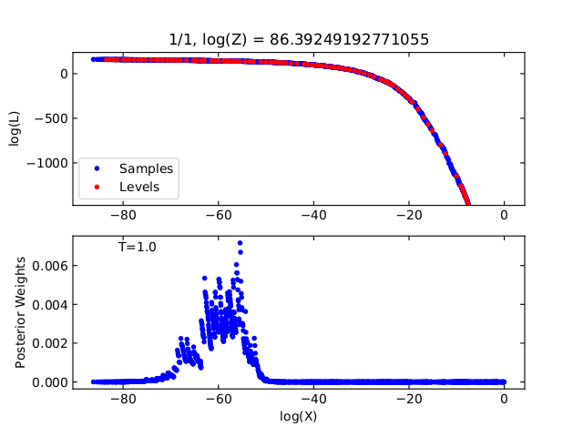
Fig.1 Example for log-likelihood cruve of a good run with appropriate options.

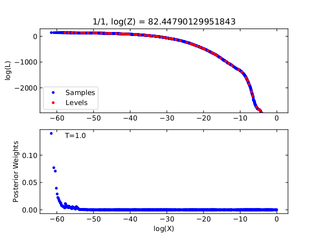
Fig.2 Example for log-likelihood cruve of a bad run with inappropriate options.